Introduction

A student in one of my classes had a bunch of latitude/longitude data from the US and wanted to map them to a US Census tract and its corresponding code (FIPS code).

We can first download the Census tracts for each state from the US Census website under the “Census Tracts” dropdown menu. Then, after unzipping the file, we can read the shape file using st_read from the sf package.

library(sf)
library(dplyr)
census_tracts <- st_read("cb_2018_42_tract_500k.shp", quiet = TRUE)

Then, we can generate some fake lat/long data for Pennsylvania.

n <- 1e5
set.seed(7477263)
county_bbox <- st_bbox(census_tracts)
# randomly sample longitude and latitude from PA's bounding box
latlong_dat <- data.frame(id = seq_len(n),
                          x = rnorm(n),
                          Longitude = runif(n, min = county_bbox["xmin"],
                                            max = county_bbox["xmax"]),
                          Latitude = runif(n, min = county_bbox["ymin"],
                                            max = county_bbox["ymax"]))

Original Solution

The original solution was to use call_geolocator_latlong to get the block FIPS using an online API, and then convert that into Census tract by taking the first 11 digits. However, the API takes a while to respond, so this solution isn’t scalable for thousands of data points.

library(tigris)
system.time({
  census_block <- tigris::call_geolocator_latlon(lat = latlong_dat$Latitude[1],
                                                 lon = latlong_dat$Longitude[1])
})

##    user  system elapsed 
##   0.059   0.004   0.602

(census_tract <- substr(census_block, start = 1, stop = 11))

## [1] "42061950500"

Improved Solution

We will use the st_intersects function from the sf library and the county-level sf shapefiles to find in which county a given lat/long pair is contained. To do that, we convert the latitude and longitude data into an sf object. Note that if you have NA values for the latitude or longitude, you’ll need to filter them out.

latlong_sf <- latlong_dat %>%
  filter(!is.na(Latitude), !is.na(Longitude)) %>%
  st_as_sf(coords = c("Longitude", "Latitude"), crs = st_crs(census_tracts))

Then, we use the st_intersects function to find the counties which intersect with the points. This returns a list, where the ith element is the row number of census_tracts which contains the ith lat/long pair.

We might get a message like:

although coordinates are longitude/latitude, st_intersects assumes that they are planar

I believe this can be ignored unless you’re working with data near the polar regions.

system.time({
  intersected <- st_intersects(latlong_sf, census_tracts)
})

##    user  system elapsed 
##   1.062   0.008   1.070

We can see that this runs super quickly—it took the same time to process all 10K lat/long pairs with st_intersects as it did to process 1 pair with call_geolocator_latlon.

We can then add the FIPS as a column to our latitude/longitude data. We can use the intersection to subset the GEOID column of census_tracts, which is the FIPS code. If the intersection was NA, then the FIPS code will be an empty string (note FIPS codes are stored as strings because sometimes they have a leading zero).

latlong_final <- latlong_sf %>%
  mutate(intersection = as.integer(intersected),
         fips = if_else(is.na(intersection), "",
                        census_tracts$GEOID[intersection]))
head(latlong_final)

## Simple feature collection with 6 features and 4 fields
## geometry type:  POINT
## dimension:      XY
## bbox:           xmin: -80.48101 ymin: 39.73635 xmax: -75.50156 ymax: 41.99468
## geographic CRS: NAD83
##   id          x                   geometry intersection        fips
## 1  1 -2.1932479 POINT (-77.89334 40.52967)         2495 42061950500
## 2  2 -2.0290433  POINT (-78.81608 41.8673)         2895 42083421000
## 3  3  0.3157029 POINT (-75.50156 39.73635)           NA            
## 4  4 -1.0549416 POINT (-80.48101 40.59035)         3154 42007602900
## 5  5  0.9947392 POINT (-78.55342 41.54438)         1774 42047950100
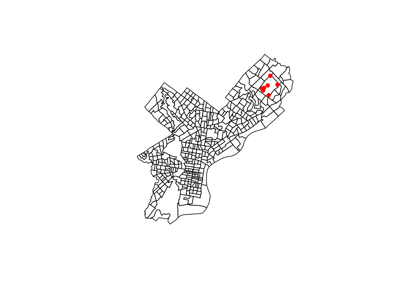
## 6  6  1.2926765 POINT (-79.69076 41.99468)         2609 42049011802

To check our solution, we can plot all the Census tracts in Philadelphia (county code 42101) and display the points which showed up in a particular Census tract.

census_tracts %>%
  filter(startsWith(GEOID, "42101")) %>%
  select(geometry) %>%
  plot()
latlong_final %>%
  filter(fips == "42101980300") %>%
  select(geometry) %>%
  slice_sample(n = 10) %>%
  plot(add = TRUE, reset = FALSE, pch = 16, col = "red")